Creating Pre-emphasis Audio CD (CD-R, technically)

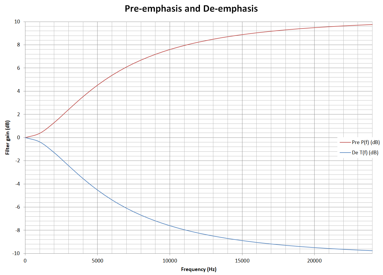
Creating FIR filter coefficients of pre-emphasis

Pre-emphasis frequency  response $P_{\mathrm{dB}}(\mathit{f})=-T_{\mathrm{dB}}(\mathit{f})$ for all frequencies $f$.
$-{\log }_{10}x={\log }_{10}\left(\left(\frac{1}{x}\right)\right)$ therefore

De-emphasis $T_{\mathrm{dB}}(\mathit{f})=10{\log }_{10}\left(\left(\frac{1+\frac{1}{{(0.000015·2\mathit{\pi }\mathit{f})}^2}}{1+\frac{1}{{(0.00005·2\mathit{\pi }\mathit{f})}^2}}\right)\right)-10.4576\dots \dots (1)$
$\mathit{f}:\; frequency\; (Hz)$
$T_{\mathrm{dB}}(\mathit{f})\; :\; De-emphasis\; filter\; gain\; (dB)$

Pre-emphasis $P_{\mathrm{dB}}(\mathit{f})=10{\log }_{10}\left(\left(\frac{1+\frac{1}{{(0.00005·2\mathit{\pi }\mathit{f})}^2}}{1+\frac{1}{{(0.000015·2\mathit{\pi }\mathit{f})}^2}}\right)\right)+10.4576\dots \dots (2)$
$\mathit{f}:\; frequency\; (Hz)$
$P_{\mathrm{dB}}(\mathit{f})\; :\; Pre-emphasis\; filter\; gain\; (dB)$

Note: Math equations of this article uses MathML and it seems it is displayed correctly only on Firefox (as of November 2020).

Now we have frequency response equation of pre-emphasis (2) and FIR filter coefficients can be calculated from  (2) using frequency sampling method, which is explained on the previous article.

Burning Audio CD-R with pre-emphasis

I used Windows PC for the following tasks.

 

Prepare Audio tracks with pre-emphasised

Prepare sound tracks of our Audio CD. 

PCM should be pre-emphasis filtered 44.1kHz 16bit WAV.

• If PCM sample rate is not 44.1kHz or audio file format is not FLAC, convert it to 44.1kHz FLAC using Audacity. https://www.audacityteam.org/download/
  
• Perform pre-emphasis to 44.1kHz 16bit or 24bit FLAC file using sox or FIRFilterConsole https://sourceforge.net/p/playpcmwin/wiki/FIRFilterConsole/
  
• Then the files should be converted from FLAC to 44.1kHz 16bit 2ch WAV using Audacity.

 I prepared the CD track WAV files Track01.wav and Track02.wav on C:\audio folder.

 

Install Cygwin and cdrecord

Download and run Cygwin setup-x86_64.exe https://www.cygwin.com/ 

Install cdrecord package: On the Select Packages menu on the Cygwin installer, Set View to "Full" and input "cdr" to Search. cdrecord package will be shown. On the pulldown list of the New column, select cdrecord version number to install.

Burn Pre-emphasis Audio data to CD-R 

Connect CD-R, DVD-R or BD-RW drive to the computer and insert CD-R.

Start → Cygwin → Cygwin64 Terminal.

Change current directory to C:\audio . Type the following text on the Cygwin64 Terminal :

$ cd /cygdrive/c/audio

Then type ls to show the file list of C:\audio folder. Make sure your wav files are there.

Create Audio CD with pre-emphasis:

$ cdrecord -audio -preemp Track01.wav Track02.wav

View Burned Audio CD-R track info using Exact Audio Copy

It seems Pre-emp is "Yes" 😄

Reading Channel status bit of S/PDIF signal from CD player

Inserted created pre-emphasis CD-R to a CD transport and played. And watched its S/PDIF signal using RME Fireface UC and found emphasis flag of channel status is "None". This means the CD transport de-emphasised PCM signal in digital domain and no further de-emphasis is necessary on receiver/DAC. 

It is possible to de-emphasis pre-emphasised PCM signal by playing it on the CD transport and recording S/PDIF signal using PCM recorder.

Pre-emphasis FIR Filter coefficients of 27 taps

This FIR filter is for 44.1kHz PCM.

-0.0001031041010544631,
3.9223988214258376E-05,
-0.00035340551190767011,
8.1196136261327267E-05,
-0.00091024157376404236,
-0.00022270417890876693,
-0.0025945766943699933,
-0.0022553226067039134,
-0.009562843431584811,
-0.015097813965845558,
-0.051492871033445048,
-0.11992388565207374,
-0.44071105358364959,
2.2862148044176558,
-0.44071105358364959,
-0.11992388565207374,
-0.051492871033445048,
-0.015097813965845558,
-0.009562843431584811,
-0.0022553226067039134,
-0.0025945766943699933,
-0.00022270417890876693,
-0.00091024157376404236,
8.1196136261327267E-05,
-0.00035340551190767011,
3.9223988214258376E-05,
-0.0001031041010544631,


Filtering sound files using sox

The following examples inputs 44.1kHz PCM file inFile.flac and apply 27taps Pre-emphasis FIR filter and output it as outFile.flac (this filter increases gain so sample value overflow may occur):

sox inFile.flac outFile.flac fir -0.0001031041010544631 3.9223988214258376E-05 -0.00035340551190767011 8.1196136261327267E-05 -0.00091024157376404236 -0.00022270417890876693 -0.0025945766943699933 -0.0022553226067039134 -0.009562843431584811 -0.015097813965845558 -0.051492871033445048 -0.11992388565207374 -0.44071105358364959 2.2862148044176558 -0.44071105358364959 -0.11992388565207374 -0.051492871033445048 -0.015097813965845558 -0.009562843431584811 -0.0022553226067039134 -0.0025945766943699933 -0.00022270417890876693 -0.00091024157376404236 8.1196136261327267E-05 -0.00035340551190767011 3.9223988214258376E-05 -0.0001031041010544631

Designing De-emphasis Digital Filter for old CDs Part 3: Using Reference Equation

 There is a reference de-emphasis equation on this page (Thanks miguelito-san) : https://forums.stevehoffman.tv/threads/cd-dat-with-pre-emphasis-how-to-de-emphasize-correctly.88541/

$T_{\mathrm{dB}}(\mathit{f})=10{\log }_{10}\left(\left(\frac{1+\frac{1}{{(0.000015·2\mathit{\pi }\mathit{f})}^2}}{1+\frac{1}{{(0.00005·2\mathit{\pi }\mathit{f})}^2}}\right)\right)-10.4576\dots \dots (1)$
$\mathit{f}:\; frequency\; (Hz)$
$T_{\mathrm{dB}}(\mathit{f})\; :\; De-emphasis\; filter\; gain\; (dB)$

This decibel is root power quantity therefore actual gain magnitude value T(f) is:

$\mathit{f}:\; frequency\; (Hz)$
$T(\mathit{f})\; :\; De-emphasis\; filter\; gain\; magnitude\; value\; at\; frequency\mathit{f}$

Note 1: Math equations of this article uses MathML and it seems it is displayed correctly only on Firefox (as of November 2020).

Note 2: It seems 0.00005 and 0.000015 of equation 1 means 50 microseconds and 15 microseconds respectively and it is called 50/15 microsec emphasis.

On this article, equation (2) is used to create frequency sampling FIR digital filter.

Calculation steps are very similar to Part 2.

Example : Calculation of M=9 taps FIR filter coeffs using equation $T(\mathit{f})$

When sampling frequency==44100 Hz and Desired FIR filter taps M==9,

Frequency sampling index $k=0,1,2,\; ..,\frac{M-1}{2}=4$

$k\; =\; 0,\; 1,\; 2,\; 3\; and\; 4$

Frequency sampling angle frequency ${\omega }_{\mathrm{k}}=\frac{2\pi k}{M}:$

• $k\; =\; 0\; :\; {\omega }_0=\; 0,\; freq0\; =\; 0\; Hz$
  
• $k\; =\; 1\; :\; {\omega }_1=\; 2\pi /9,\; freq1\; =\; (44100/2\pi )(2\pi /9)\; =\; 44100\; /\; 9\; Hz\; =\; 4900\; Hz$
• $k\; =\; 2\; :\; {\omega }_2=\; 4\pi /9,\; freq2\; =\; (44100/2\pi )(4\pi /9)\; =\; 44100\; *\; 2\; /\; 9\; Hz\; =\; 9800\; Hz$
• $k\; =\; 3\; :\; {\omega }_3=\; 6\pi /9,\; freq3\; =\; (44100/2\pi )(6\pi /9)\; =\; 44100\; *\; 3\; /\; 9\; Hz\; =\; 14700\; Hz$
• $k\; =\; 4\; :\; {\omega }_4=\; 8\pi /9,\; freq4\; =\; (44100/2\pi )(8\pi /9)\; =\; 44100\; *\; 4\; /\; 9\; Hz\; =\; 19600\; Hz$

Get filter gain on those frequencies $Hr({\omega }_{\mathrm{k}})$ using Equation (2):

• $Hr($ {\omega }_0)\; =\; T(0)\; =\; 1$$
• $Hr($ {\omega }_1)\; =\; T(4900)\; =\; 0.60004356$$
• $Hr($ {\omega }_2)\; =\; T(9800)\; =\; 0.420524967$$
• $Hr($ {\omega }_3)\; =\; T(14700)\; =\; 0.361602897$$
• $Hr($ {\omega }_4)\; =\; T(19600)\; =\; 0.336724814$$

Then G(k) is calculated from $Hr({\omega }_{\mathrm{k}})$ by $G(k)\; ={\mathrm{(-1)}}^{\mathrm{k}}Hr($ {\omega }_{\mathrm{k}})\; \dots \dots (3)\; :$$

• $G(0)\; ={\mathrm{(-1)}}^{0}Hr($ {\omega }_0)\; =\; 1$$
• $G(1)\; ={\mathrm{(-1)}}^{1}Hr($ {\omega }_1)\; =\; -0.60004356$$
• $G(2)\; ={\mathrm{(-1)}}^{2}Hr($ {\omega }_2)\; =\; 0.420524967$$
• $G(3)\; ={\mathrm{(-1)}}^{3}Hr($ {\omega }_3)\; =\; -0.361602897$$
• $G(4)\; ={\mathrm{(-1)}}^{4}Hr($ {\omega }_4)\; =\; 0.336724814$$

FIR filter coefficients h(n) can be calculated by $h(n)\; =\frac{1}{M}\left\{G(0)+2\sum _{\mathrm{k=1}}^{\mathrm{(M-1)/2}}G(k)cos\frac{2\pi k(n+1/2)}{M}\right\}\dots (4)$

• $h(0)\; =\; 0.030212113446082472$
• $h(1)\; =\; 0.040656939222222181$
• $h(2)\; =\; 0.063594885887469199$
• $h(3)\; =\; 0.11899203499978166$
• $h(4)\; =\; 0.49308805288888891$

Finally, this FIR filter is symmetry (linear phase), therefore h(8) = h(0), h(7) = h(1), h(6) = h(2), h(5) = h(3).

• $h(0)\; =\; 0.030212113446082472$
• $h(1)\; =\; 0.040656939222222181$
• $h(2)\; =\; 0.063594885887469199$
• $h(3)\; =\; 0.11899203499978166$
• $h(4)\; =\; 0.49308805288888891$
• $h(5)\; =\; 0.11899203499978166$
• $h(6)\; =\; 0.063594885887469199$
• $h(7)\; =\; 0.040656939222222181$
• $h(8)\; =\; 0.030212113446082472$

We've got all the 9 FIR filter coefficients h(n).

Evaluating Frequency Response of FIR filter

Now one FIR filter is available for testing. FIR filter gain of arbitrary angular frequency ω can be calculated using the following equation:

$Gain(\omega )\; =\sum _{\mathrm{k=0}}^{\mathrm{M-1}}h(k)e^{\mathrm{-jk\omega }}\dots \dots (5)$

Real part and imaginary part of (5) can be calculated separately:

${\mathrm{Gain}}_{\mathrm{real}}(\omega )\; =\sum _{\mathrm{k=0}}^{\mathrm{M-1}}h(k)cos(-k\omega )\; \dots \dots (5r)$
${\mathrm{Gain}}_{\mathrm{imaginary}}(\omega )\; =\sum _{\mathrm{k=0}}^{\mathrm{M-1}}h(k)sin(-k\omega )\; \dots \dots (5i)$

And FIR filter Gain magnitude is calculated as follows:

Finally Gain in decibel is: ${\mathrm{Gain}}_{\mathrm{dB}}(\omega )\; =\; 20{\log }_{10}\left\{{\mathrm{Gain}}_{\mathrm{magnitude}}(\omega )\right\}\dots \dots (7)$

For our M=9 FIR filter, frequency response can be calculated using equation (7). And this time reference equation is available: desirable gain of any frequency can be calculated, it is possible to compare gain values at as many frequency points as you wish. I compared 10Hz to 22040Hz semitone step frequency points and created Fig.1.

Fig.1. 9 taps FIR de-emphasis filter frequency response.

Comparing to the original de-emphasis table, max error of this FIR filter is 0.878 dB on 7360Hz, It is poor, and the quality can be improved by increasing M.

Searching the best FIR filter tap number M

FIR Filter Taps M	Max Error (dB)
9	0.878
15	0.1704
17	0.115
19	0.0631
21	0.0522
23	0.0231
25	0.0272
27	0.00882

Table 1: FIR Filter taps and max error 

Fig.2 : Frequency Response of FIR Filter, taps=19  note: frequency axis is logarithmic.

Fig.3 : Frequency Response of FIR Filter, taps=27  note: frequency axis is logarithmic.

Fig.4 : Gain Error of FIR Filter, taps=27

De-emphasis FIR Filter Coefficients for 44.1kHz PCM data

19taps linear-phase FIR filter coefficients h(n) of max error = 0.0631 dB is as follows:

0.0022333652179533105,
0.0027676001211334594,
0.0042218013139663415,
0.0065438712761329912,
0.011312237381544295,
0.01877355043394098,
0.03398288954901494,
0.059120380386441337,
0.11593361915957012,
0.49022137032060437,
0.11593361915957012,
0.059120380386441337,
0.03398288954901494,
0.01877355043394098,
0.011312237381544295,
0.0065438712761329912,
0.0042218013139663415,
0.0027676001211334594,
0.0022333652179533105,

27taps linear-phase FIR filter coefficients h(n) of max error = 0.00882 dB is as follows:

0.00031102739649091732,
0.00036885685453166665,
0.00057659816229764602,
0.00082952248115418167,
0.001449970925925961,
0.0022387507393955598,
0.0039420948394406248,
0.0063363475292175873,
0.011215231698621361,
0.018685854350970088,
0.033951734838472802,
0.059076192885731141,
0.11592376177923121,
0.49018811103703697,
0.11592376177923121,
0.059076192885731141,
0.033951734838472802,
0.018685854350970088,
0.011215231698621361,
0.0063363475292175873,
0.0039420948394406248,
0.0022387507393955598,
0.001449970925925961,
0.00082952248115418167,
0.00057659816229764602,
0.00036885685453166665,
0.00031102739649091732,

Filtering sound files using sox

With sox, it is possible to use those coefficients to filter the 44.1kHz PCM sound files. The following examples inputs inFile.flac and apply 27taps De-emphasis FIR filter and output it as outFile.flac:

sox inFile.flac outFile.flac fir 0.00031102739649091732 0.00036885685453166665 0.00057659816229764602 0.00082952248115418167 0.001449970925925961 0.0022387507393955598 0.0039420948394406248 0.0063363475292175873 0.011215231698621361 0.018685854350970088 0.033951734838472802 0.059076192885731141 0.11592376177923121 0.49018811103703697 0.11592376177923121 0.059076192885731141 0.033951734838472802 0.018685854350970088 0.011215231698621361 0.0063363475292175873 0.0039420948394406248 0.0022387507393955598 0.001449970925925961 0.00082952248115418167 0.00057659816229764602 0.00036885685453166665 0.00031102739649091732

Next article: Creating Pre-emphasis Audio CD

Designing De-emphasis Digital Filter for Old CDs Part 2 : Frequency Sampling Method

On the previous blog post, we've got a 6th degree polynomial function of de-emphasis curve Equation 1:

$f\mathrm{dB}(x)\; =\; -0.0000029212346025337816x^6+0.00020291497408909238x^5-0.0054888099286801205x^4+0.071110615465301924x^3-0.40078216359333169x^2-0.11354738870338571x$

$x\; :\; frequency\; (kHz)$
$f_{\mathrm{dB}}(x):\; filter\; gain\; (dB)$

Note: Math equations of this article uses MathML and it seems it is displayed correctly only on Firefox (as of November 2020).

This decibel is root power quantity therefore actual gain value f(x) is:

Next step is to create filter gain table of equal spacing frequency using this function.

And create the filter, evaluate its frequency response error from original de-emphasis table and choose the best FIR filter tap number M.

 

Example : Calculation of M=9 taps FIR filter coeffs

When sampling frequency==44100 Hz and Desired FIR filter taps M==9,

Frequency sampling index $k=0,1,2,\; ..,\frac{M-1}{2}=4$

$k=0,1,2,3\; and\; 4$

Frequency sampling angle frequency ${\omega }_{\mathrm{k}}=\frac{2\pi k}{M}:$

• $k=0: {\omega }_0=\; 0, {\mathrm{freq}}_0=\; 0\; Hz$
  
• $k=1: {\omega }_1=\; 2\pi /9, {\mathrm{freq}}_1=\; (44100/2\pi )(2\pi /9)\; =\; 44100\; /\; 9\; Hz\; =\; 4900\; Hz$
• $k=2: {\omega }_2=\; 4\pi /9, {\mathrm{freq}}_2=\; (44100/2\pi )(4\pi /9)\; =\; 44100\; *\; 2\; /\; 9\; Hz\; =\; 9800\; Hz$
• $k=3: {\omega }_3=\; 6\pi /9, {\mathrm{freq}}_3=\; (44100/2\pi )(6\pi /9)\; =\; 44100\; *\; 3\; /\; 9\; Hz\; =\; 14700\; Hz$
• $k=4: {\omega }_4=\; 8\pi /9, {\mathrm{freq}}_4=\; (44100/2\pi )(8\pi /9)\; =\; 44100\; *\; 4\; /\; 9\; Hz\; =\; 19600\; Hz$

Get filter gain on those frequencies $Hr({\omega }_{\mathrm{k}})$ using Equation (2):

• $Hr({\omega }_0)\; =\; f(0)\; =\; 1$
• $Hr({\omega }_1)\; =\; f(4.9)\; =\; 0.599479869$
• $Hr({\omega }_2)\; =\; f(9.8)\; =\; 0.419371436$
• $Hr({\omega }_3)\; =\; f(14.7)\; =\; 0.359695479$
• $Hr({\omega }_4)\; =\; f(19.6)\; =\; 0.33620803$

Then G(k) is calculated from $Hr({\omega }_{\mathrm{k}})$ by $G(k)\; ={\mathrm{(-1)}}^{\mathrm{k}}Hr({\omega }_{\mathrm{k}})\; \dots \dots (3)\; :$

• $G(0)\; ={\mathrm{(-1)}}^{0}Hr({\omega }_0)\; =\; 1$
• $G(1)\; ={\mathrm{(-1)}}^{1}Hr({\omega }_1)\; =\; -0.599479869$
• $G(2)\; ={\mathrm{(-1)}}^{2}Hr({\omega }_2)\; =\; 0.419371436$
• $G(3)\; ={\mathrm{(-1)}}^{3}Hr({\omega }_3)\; =\; -0.359695479$
• $G(4)\; ={\mathrm{(-1)}}^{4}Hr({\omega }_4)\; =\; 0.33620803$

FIR filter coefficients h(n) can be calculated by $h(n)\; =\frac{1}{M}\left\{G(0)+2\sum _{\mathrm{k=1}}^{\mathrm{(M-1)/2}}G(k)cos\frac{2\pi k(n+1/2)}{M}\right\}\dots (4)$

• $h(0)\; =\; 0.0303254491484693$
• $h(1)\; =\; 0.0404812914444444$
• $h(2)\; =\; 0.0639379770301665$
• $h(3)\; =\; 0.119171414154698$
• $h(4)\; =\; 0.492167736444444$

And finally, This FIR filter is symmetry shape, therefore h(8) = h(0), h(7) = h(1), h(6) = h(2), h(5) = h(3).

• $h(0)\; =\; 0.0303254491484693$
• $h(1)\; =\; 0.0404812914444444$
• $h(2)\; =\; 0.0639379770301665$
• $h(3)\; =\; 0.119171414154698$
• $h(4)\; =\; 0.492167736444444$
• $h(5)\; =\; 0.119171414154698$
• $h(6)\; =\; 0.0639379770301665$
• $h(7)\; =\; 0.0404812914444444$
• $h(8)\; =\; 0.0303254491484693$

We've got all the 9 FIR coefficient values h(n).

Evaluating Frequency Response of FIR filter

Now one FIR filter coefficients h(n) is available for testing. FIR filter gain of arbitrary angular frequency ω can be calculated using the following equation:

$Gain(\omega )\; =\sum _{\mathrm{k=0}}^{\mathrm{M-1}}h(k)e^{\mathrm{-jk\omega }}\dots \dots (5)$

Real part and imaginary part of (5) can be calculated separately:

${\mathrm{Gain}}_{\mathrm{real}}(\omega )\; =\sum _{\mathrm{k=0}}^{\mathrm{M-1}}h(k)cos(-k\omega )\; \dots \dots (5r)$
${\mathrm{Gain}}_{\mathrm{imaginary}}(\omega )\; =\sum _{\mathrm{k=0}}^{\mathrm{M-1}}h(k)sin(-k\omega )\; \dots \dots (5i)$

And FIR filter Gain magnitude is calculated as follows:

Finally Gain in decibel is: ${\mathrm{Gain}}_{\mathrm{dB}}(\omega )\; =\; 20{\log }_{10}\left\{{\mathrm{Gain}}_{\mathrm{magnitude}}(\omega )\right\}\dots \dots (7)$

For our M=9 FIR filter, frequency response can be calculated using equation (7):

Frequency(kHz)	${\mathrm{Gain}}_{\mathrm{dB}}(\omega )$
0	0
1	-0.214929748
2	-0.847460501
3	-1.855702469
4	-3.153141013
5	-4.58835657
6	-5.939107409
7	-6.960958392
8	-7.506314657
9	-7.624120111
10	-7.521831664
11	-7.433783042
12	-7.52486218
13	-7.862458657
14	-8.419180318
15	-9.081142015
16	-9.670162018
17	-10.00514702
18	-9.997371674
19	-9.707880014
20	-9.30607583
21	-8.974681539
22	-8.840811148

Table 1

Comparing to the original de-emphasis table, max error of this FIR filter is 0.87 dB on 7kHz, It is poor and may be M=9 is too small.

Finding Optimal FIR filter taps M

I'd like to have < 0.1 dB error of FIR filter with minimum filter taps. Calculated error from the original table on several M using DesignFrequencySamplingFilter and compared their performance.

Filter taps M	Max error from the original table
9	0.871 dB
17	0.217 dB
19	0.140 dB
21	0.172 dB
23	0.104 dB
25	0.118 dB
27	0.0779 dB
29	0.0802 dB
31	0.0795 dB
33	0.0770 dB

Table 2

From the table 2, M=27 is the most desirable one.

On M=27,  maximum error from the original table is 0.0779 dB on 2kHz.

Resulted linear-phase FIR filter coefficients h(n) of M=27 for 44.1kHz PCM is as follows:

0.00087829953598830856,
0.00073354073461322569,
0.0013059505528472161,
0.00089158366884379073,
0.0022743712962963354,
0.0017509721612062167,
0.0046856769010995523,
0.0049418323357026065,
0.011621996337245248,
0.017825153275235591,
0.034805918374128435,
0.057946349576219941,
0.11652885832464696,
0.48761899385185181,
0.11652885832464696,
0.057946349576219941,
0.034805918374128435,
0.017825153275235591,
0.011621996337245248,
0.0049418323357026065,
0.0046856769010995523,
0.0017509721612062167,
0.0022743712962963354,
0.00089158366884379073,
0.0013059505528472161,
0.00073354073461322569,
0.00087829953598830856

Fig.1 M=27 de-emphasis FIR Filter frequency response

This linear-phase de-emphasis FIR filter is available on DSP menu of PlayPcmWin 5.0.79. Source code is https://sourceforge.net/p/playpcmwin/code/HEAD/tree/PlayPcmWin/WasapiIODLL/WWAudioFilterDeEmphasis.cpp

 

Continued to Part 3 (Improving accuracy): https://yamamoto2002.blogspot.com/2020/11/designing-de-emphasis-digital-filter.html

 

 Reference

 J.G. Proakis & D.G. Manolakis: Digital Signal Processing, 4th edition, 2007, Chapter 10, pp. 671-678

Designing De-emphasis Digital Filter for Old CDs Part 1: Polynomial Fitting

 
I have one pre-emphasis CD and ripped it to FLAC files. In order to play it correctly, de-emphasis is necessary. So started to design de-emphasis filter for 44.1kHz PCM.

There are many ways to design filters. I chose frequency-sampling method to create linear-phase FIR filter.

De-emphasis filter curve

From the following page, there is a frequency response table: https://archimago.blogspot.com/2020/09/how-to-cd-pre-emphasis-and-dealing-with.html

f(Hz)	De-emphasis filter gain (dB)
0	0
1	-0.37
2	-1.29
3	-2.43
4	-3.54
5	-4.53
6	-5.38
7	-6.09
8	-6.69
9	-7.19
10	-7.6
11	-7.95
12	-8.24
13	-8.49
14	-8.71
15	-8.89
16	-9.04
17	-9.18
18	-9.3
19	-9.4
20	-9.49

Table 1 De-emphasis filter frequency response

Polynomial fitting

In order to design the filter, it is necessary to know the filter gain of arbitrary frequency. So I tried Excel polynomial fit to find the best polynomial equation.

Note: this process is not necessary, because reference frequency response function is available: https://yamamoto2002.blogspot.com/2020/11/designing-de-emphasis-digital-filter.html

Fig.1 line fitting

Fig.2 2nd degree polynomial fit

Fig.3 3rd degree polynomial fit

Fig.4 4th degree polynomial fit

Fig.5 5th degree polynomial fit

Fig.6 6th degree polynomial fit

From the graphs above, 6th degree polynomial is the best and I decided to use it. other functions have a problem on the 0Hz～2kHz region, and its frequency band is very important for music. the error can be reduced further by increasing polynomial degree but I think < 0.1 dB is sufficient.

Calculating Polynomial coefficient

Excel shows 6th degree polynomial coefficient values on Fig.6, but it is ballpark values and more precise coefficient values are needed. Polynomial fit code WWPolynomialFit.cs to get 6th polynomial coefficient values.

Result is:

constant	1st	2nd	3rd	4th	5th	6th
0.028327961846712043	-0.11354738870338571	-0.40078216359333169	0.071110615465301924	-0.0054888099286801205	0.00020291497408909238	-0.0000029212346025337816

Table 2. 6th degree polynomial coefficients

There is a very small constant value but it should be 0 to prevent PCM integer overflow, so I just modified constant coefficient to zero.

Resulted equation is:

$y=\; -0.0000029212346025337816x^6+0.00020291497408909238x^5-0.0054888099286801205x^4+0.071110615465301924x^3-0.40078216359333169x^2-0.11354738870338571x\; \dots \dots (1)$
$x\; :\; Frequency\; (kHz)$
$y\; :\; Filter\; gain\; (dB)$

Note: Math equations of this article uses MathML and it seems it is displayed correctly only on Firefox (as of November 2020).

Error from the table values are: 0.079 dB on 1kHz, 0.053 dB on 2kHz, and so on.

Now it is possible to get the filter gain at arbitrary frequency using the equation (1).

Continued to Part 2: https://yamamoto2002.blogspot.com/2020/11/designing-de-emphasis-fir-filter-for.html

Creating Music Key predictor AI

Motivation

I purchased Scott Ross Scarlatti CD box that contains all the Scarlatti keyboard sonatas.

Listened to a few pieces and found they modulate frequently and I'd like to know what key is played on now.

 

Creating training data for 24 key classifier Linear Support Vector Machine

Rip Scarlatti Scott Ross CDs from K1 to K100 to create K1.flac to K100.flac

The harpsichord is tuned in baroque pitch. I'm not good at inspecting the key of baroque pitch so pitch is increased by semitone to concert pitch using WWArbitraryResampler. And convert them to monaural WAV and store on WAV_Reference directory for AI training.

WWArbitraryResampler: https://sourceforge.net/p/playpcmwin/wiki/WWArbitraryResampler/

Listen to FLAC of concert pitch files from K1 to K100 and roughly write down time and key: https://sourceforge.net/p/playpcmwin/code/HEAD/tree/PlayPcmWin/WWKeyClassifier2/train/Keys_faithful.csv

On K25,  Cisdur appears but it is changed to Desdur (to converge number of keys to 24). 

Create harpsichord key press data for learning. FFT with 16384 window length and extract 110Hz (A2) to 1318.5Hz (E6) frequency components by semitone step (Fig.1). harpsichod have several lower keys, but lower key press info is blurred and spread to adjacent keys so I decided to exclude them.

Fig.1: harpsichord keys.

 
On Matlab, run classificationLearner() and input spectral component data of 24 keys music snippets and learn LinearSVM to create linear SVM model and export C# Linear SVM coefficients. 

Resulted classifier code:

https://sourceforge.net/p/playpcmwin/code/HEAD/tree/PlayPcmWin/WWKeyClassifier2/KeyClassifierCore.cs 

Created app, WWKeyClassifier2:

https://sourceforge.net/p/playpcmwin/wiki/WWKeyClassifier2/

 

Fig.2 WWKeyClassifier App

Accuracy of the SVM classifier

There are 24 keys categories to be classified. 12 major keys and 12 minor keys.

Combination(24,2) = 276 one-by-one Binary Classifier is created from the training. For example, Cdur-Cmoll classifier can tell is input music Cdur or Cmoll,  there is Cdur-Amoll classifier, Cdur-Gdur classifier and so on.

Prediction accuracy is about 80%. It seems Hdur tends to falsely classified as Edur.

Table 1 : confusion matrix of the 24 keys classifier.

What the AI learned from the training

Following is the`beta' coefficient table of Cdur-Cmoll binary linear SVM classifier. This table means: when E note is appeared, it is probably Cdur. When Es (Dis in the following graph) note is appeared, it is probably Cmoll. This is somewhat understandable. 

 

When the music is found to be either Cdur or Cmoll,

• E note is appeared→ it is probably Cdur.
• Es note is appeared→ it is probably Cmoll.

AI automatically obtained this knowledge from `Scarlatti listening' training 😀I'm envious of computers that have an absolute pitch.

 Table 2: Cdur-Cmoll binary classifier beta coefficients.

Table 3: Cdur-Amoll classifier. G note→Cdur, Gis note→Amoll.

Table 4: Cdur-Gdur classifier. Fis note→Gdur. F note→Cdur. E note→may be Cdur.

 

 

Table 5: Cdur-Fdur classifier. H note→Cdur, B note→Fdur. D note→may be Cdur. A note→may be Fdur.

Table 6: Hdur-Edur classifier. A note→Edur, Ais note→Hdur. Cis note→may be Hdur. Gis note→may be Edur. There is no apparent flaw seen on this chart but this classifier tends to falsely classify Hdur music as Edur.

Table 7: Cdur-Fisdur classifier. This is easy job. Computer never mis-classify Cdur music as Fisdur because those two keys are very different.

About Voting

There are Combination(24,2) = 276 binary classifiers, each classifier tells which key is more probable with given two keys. For example, Desdur-Cdur classifier tells inputted data is Desdur or Cdur. When one FFT data is inputted, our Multiclass Classifier runs 276 binary classifiers and choose most voted key as a result.

For example, this process creates something like the following table and "Dmoll" is chosen as a most probable result. From the table, it seems the next candidate is Adur and Ddur.

-

Cdur

Desdur

Ddur

Esdur

Edur

Fdur

Fisdur

Gdur

Asdur

Adur

Bdur

Hdur

Cmoll

Cismoll

Dmoll

Dismoll

Emoll

Fmoll

Fismoll

Gmoll

Gismoll

Amoll

Bmoll

Hmoll

Cdur

-

-

-

-

-

-

-

-

-

-

-

-

-

-

-

-

-

-

-

-

-

-

-

-

Desdur

Cdur

-

-

-

-

-

-

-

-

-

-

-

-

-

-

-

-

-

-

-

-

-

-

-

Ddur

Ddur

Ddur

-

-

-

-

-

-

-

-

-

-

-

-

-

-

-

-

-

-

-

-

-

-

Esdur

Cdur

Esdur

Ddur

-

-

-

-

-

-

-

-

-

-

-

-

-

-

-

-

-

-

-

-

-

Edur

Cdur

Edur

Ddur

Edur

-

-

-

-

-

-

-

-

-

-

-

-

-

-

-

-

-

-

-

-

Fdur

Fdur

Fdur

Ddur

Fdur

Fdur

-

-

-

-

-

-

-

-

-

-

-

-

-

-

-

-

-

-

-

Fisdur

Cdur

Desdur

Ddur

Esdur

Edur

Fdur

-

-

-

-

-

-

-

-

-

-

-

-

-

-

-

-

-

-

Gdur

Gdur

Gdur

Ddur

Gdur

Gdur

Fdur

Gdur

-

-

-

-

-

-

-

-

-

-

-

-

-

-

-

-

-

Asdur

Cdur

Asdur

Ddur

Esdur

Edur

Fdur

Asdur

Gdur

-

-

-

-

-

-

-

-

-

-

-

-

-

-

-

-

Adur

Adur

Adur

Ddur

Adur

Adur

Adur

Adur

Adur

Adur

-

-

-

-

-

-

-

-

-

-

-

-

-

-

-

Bdur

Cdur

Bdur

Ddur

Bdur

Edur

Fdur

Bdur

Gdur

Bdur

Adur

-

-

-

-

-

-

-

-

-

-

-

-

-

-

Hdur

Cdur

Hdur

Ddur

Esdur

Edur

Fdur

Hdur

Gdur

Asdur

Adur

Bdur

-

-

-

-

-

-

-

-

-

-

-

-

-

Cmoll

Cdur

Cmoll

Ddur

Cmoll

Cmoll

Fdur

Cmoll

Gdur

Cmoll

Adur

Bdur

Cmoll

-

-

-

-

-

-

-

-

-

-

-

-

Cismoll

Cdur

Cismoll

Ddur

Esdur

Edur

Fdur

Cismoll

Gdur

Cismoll

Adur

Bdur

Cismoll

Cmoll

-

-

-

-

-

-

-

-

-

-

-

Dmoll

Dmoll

Dmoll

Dmoll

Dmoll

Dmoll

Dmoll

Dmoll

Dmoll

Dmoll

Dmoll

Dmoll

Dmoll

Dmoll

Dmoll

-

-

-

-

-

-

-

-

-

-

Dismoll

Cdur

Dismoll

Ddur

Esdur

Edur

Fdur

Dismoll

Gdur

Dismoll

Adur

Bdur

Dismoll

Cmoll

Cismoll

Dmoll

-

-

-

-

-

-

-

-

-

Emoll

Cdur

Emoll

Ddur

Emoll

Emoll

Fdur

Emoll

Gdur

Emoll

Adur

Emoll

Emoll

Cmoll

Emoll

Dmoll

Emoll

-

-

-

-

-

-

-

-

Fmoll

Cdur

Fmoll

Ddur

Fmoll

Edur

Fdur

Fmoll

Gdur

Fmoll

Adur

Bdur

Fmoll

Cmoll

Fmoll

Dmoll

Fmoll

Emoll

-

-

-

-

-

-

-

Fismoll

Cdur

Fismoll

Ddur

Esdur

Edur

Fdur

Fismoll

Gdur

Fismoll

Adur

Bdur

Fismoll

Cmoll

Fismoll

Dmoll

Fismoll

Fismoll

Fismoll

-

-

-

-

-

-

Gmoll

Cdur

Gmoll

Ddur

Gmoll

Gmoll

Fdur

Gmoll

Gdur

Gmoll

Adur

Gmoll

Gmoll

Gmoll

Gmoll

Dmoll

Gmoll

Gmoll

Gmoll

Gmoll

-

-

-

-

-

Gismoll

Cdur

Gismoll

Ddur

Esdur

Edur

Fdur

Gismoll

Gdur

Asdur

Adur

Bdur

Hdur

Cmoll

Cismoll

Dmoll

Dismoll

Emoll

Fmoll

Fismoll

Gmoll

-

-

-

-

Amoll

Cdur

Amoll

Ddur

Amoll

Edur

Amoll

Amoll

Gdur

Amoll

Adur

Amoll

Amoll

Amoll

Amoll

Dmoll

Amoll

Amoll

Amoll

Amoll

Amoll

Amoll

-

-

-

Bmoll

Cdur

Bmoll

Ddur

Esdur

Edur

Fdur

Bmoll

Gdur

Bmoll

Adur

Bdur

Bmoll

Cmoll

Cismoll

Dmoll

Bmoll

Emoll

Fmoll

Fismoll

Gmoll

Bmoll

Amoll

-

-

Hmoll

Cdur

Hmoll

Ddur

Hmoll

Hmoll

Fdur

Hmoll

Gdur

Hmoll

Adur

Hmoll

Hmoll

Hmoll

Hmoll

Dmoll

Hmoll

Hmoll

Hmoll

Hmoll

Hmoll

Hmoll

Amoll

Hmoll

-

Running Simple DirectX12 Compute Shader: Looking into Dispatch xyz, numthreads xyz, SV_GroupIndex and SV_GroupID xyz

There are many arguments to run compute shader and many arguments are passed to compute shader main function.

On this post, a computer shader is executed with

• Dispatch(4,1,1)
• numthreads(3,1,1)

to see what argument values are passed to compute shader main function.

Source code

Project direcory: https://sourceforge.net/p/playpcmwin/code/HEAD/tree/PlayPcmWin/WWDirectCompute12Test2019/

Compute shader: https://sourceforge.net/p/playpcmwin/code/HEAD/tree/PlayPcmWin/WWDirectCompute12Test2019/Sandbox.hlsl

C++ program to run the compute shader: https://sourceforge.net/p/playpcmwin/code/HEAD/tree/PlayPcmWin/WWDirectCompute12Test2019/TestSandboxShader.cpp

Compute shader to run on the GPU

Sandbox.hlsl : this compute shader is called with Dispatch(4,1,1)

RWStructuredBuffer<float> g_output   : register(u0);

[numthreads(3, 1, 1)]
void
CSMain(
    uint tid : SV_GroupIndex,                 // 0 <= tid < 3 ← numthreads(3,1,1)
    uint3 groupIdXYZ : SV_GroupID)   // 0 <= groupIdXYZ.x < 4 ← Dispatch(xyz=(4,1,1))
{
    int idx = tid + groupIdXYZ.x * 5;
    g_output[idx] = 1;
}

Shader setup

Please refer TestSandboxShader.cpp. It compiles Sandbox.hlsl as a compute shader, prepares GPU buffer of 4096 bytes and sets Unordered Access View, creates compute state, calls Dispatch(4,1,1), and copy GPU buffer memory values to CPU memory of float array.

Compute Shader resources, shader main function arguments and thread group

Unordered Access View u0 is visible from the compute shader. Shader can read/write to this buffer.

CSMain function is called 12 times total, function argument of each call is as follows:

CSMain(tid=0, groupIdXYZ=0,0,0)

CSMain(tid=1, groupIdXYZ=0,0,0)
CSMain(tid=2, groupIdXYZ=0,0,0)

CSMain(tid=0, groupIdXYZ=1,0,0)
CSMain(tid=1, groupIdXYZ=1,0,0)
CSMain(tid=2, groupIdXYZ=1,0,0)

CSMain(tid=0, groupIdXYZ=2,0,0)
CSMain(tid=1, groupIdXYZ=2,0,0)
CSMain(tid=2, groupIdXYZ=2,0,0)

CSMain(tid=0, groupIdXYZ=3,0,0)
CSMain(tid=1, groupIdXYZ=3,0,0)
CSMain(tid=2, groupIdXYZ=3,0,0)

3 subsequent calls share the same groupIdXYZ and those 3 calls are executed "simultaneously": GPU has several hundred cores. 3 tasks are assigned to 3 individual GPU cores and they runs in parallel (See the following image). On more practical compute shader, it is important to run 128 or more shaders in parallel: something like numthreads(128,1,1) to utilize GPU cores fully.

Those 3 function calls that shares the same groupIdXYZ is called the thread group. GPU function calls of the same thread group can share thread group shared memory (TGSM) that is significantly faster than UAV memory, while TGSM size is limited to 32 KB or so. Utilizing TGSM is one of the key technique to accelerate GPU computation.

On this Sandbox compute shader, each shader writes adjacent GPU memory position simultaneously. This slows down write operation. It is better for each threadgroup threads to write to more remote memory position each other to write data more quickly.

Values written to u0 GPU memory

Sandbox.hlsl shader writes those values to the GPU buffer memory u0:g_Output.

    i, g_output[i], Shader function args to write this value

    0, 1.000000,   <== CSMain(tid=0, groupIdXYZ=0,0,0)
    1, 1.000000,   <== CSMain(tid=1, groupIdXYZ=0,0,0)
    2, 1.000000,   <== CSMain(tid=2, groupIdXYZ=0,0,0)
    3, 0.000000,
    4, 0.000000,
    5, 1.000000,   <== CSMain(tid=0, groupIdXYZ=1,0,0)
    6, 1.000000,   <== CSMain(tid=1, groupIdXYZ=1,0,0)
    7, 1.000000,   <== CSMain(tid=2, groupIdXYZ=1,0,0)
    8, 0.000000,
    9, 0.000000,
   10, 1.000000,   <== CSMain(tid=0, groupIdXYZ=2,0,0)
   11, 1.000000,   <== CSMain(tid=1, groupIdXYZ=2,0,0)
   12, 1.000000,   <== CSMain(tid=2, groupIdXYZ=2,0,0)
   13, 0.000000,
   14, 0.000000,
   15, 1.000000,   <== CSMain(tid=0, groupIdXYZ=3,0,0)
   16, 1.000000,   <== CSMain(tid=1, groupIdXYZ=3,0,0)
   17, 1.000000,   <== CSMain(tid=2, groupIdXYZ=3,0,0)
   18, 0.000000,
   19, 0.000000,
   20, 0.000000,
   21, 0.000000,
   22, 0.000000,
   23, 0.000000,
   24, 0.000000,